
Preprocessed Datasets
Welcome to the preprocessed datasets module!
In this module, we will learn about the different ways to navigate through the plethora of datasets available in GEE.
GEE offers easy access to millions of images from the entire lifetime of numerous imaging satellites! These large collections can be difficult to work with, which makes it daunting to find the ones you need. But fear not! We'll show you the easiest ways to navigate through the GEE data catalog and find the dataset you're looking for. We will also explore some pre-made datasets that are available to us, specifically for the tracks of this hackathon!
“In the age of big data, it’s easy to feel like a needle in a haystack. But sometimes, the haystack is the dataset.”
Navigating EE datasets
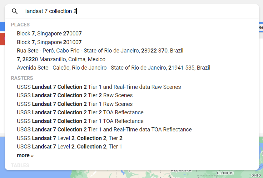
Start by typing "Landsat 7 Collection 2" in the search bar of the Earth Engine Code Editor.
You may select a dataset from this initial dropdown, or hit enter to view all search results. From there, let's look at the "USGS Landsat 7 Collection 2 Tier 1 Raw Scenes" shown to the right.
Clicking on said dataset will yield the information box also shown to the right. Here, we can see information about the dataset, including a description, bands that are available, image properties, and terms of use for the data across the top. On the left-hand side of this window, you will see a range of dates when the data is available, a link to the dataset provider’s webpage, and a collection snippet. This collection snippet can be used to import the dataset by pasting it into your script, as you did in previous chapters. You can also use the large Import button to import the dataset into your current workspace. In addition, if you click on the See example link, Earth Engine will open a new code window with a snippet of code that shows code using the dataset. Code snippets like this can be very helpful when learning how to use a dataset that is new to you.
Now navigate back to your Search Results. In the bottom right corner, click Open in Catalog. This yields an alternate view of the available data.

Data preprocessing
Let’s go over some more basics that will be useful throughout the hackathon. You can’t analyze any satellite images if you don’t have the images to start with, right?
Viewing a Landsat image collection
Depending on how long a remote sensing platform has been in operation, there may be thousands or millions of images collected of Earth. In Earth Engine, these are organized into an ImageCollection, a specialized data type that has specific operations available in the Earth Engine API. Like individual images, they can be viewed with Map.addLayer.
The Landsat program from NASA and the USGS has launched a sequence of Earth observation satellites that have been returning images since 1972, making that collection of images the longest satellite-based observation of the Earth's surface. Let's view collections of scenes taken by the Operational Land Imager aboard Landsat 8, which was launched in 2013. (Note, you do not have to run this code as it will take a long time, just follow along to understand that imageCollections may be huge!)
 /////
// View an Image Collection
/////

// Import the Landsat 8 Raw Collection.
var landsat8 = ee.ImageCollection('LANDSAT/LC08/C02/T1');

// Print the size of the Landsat 8 dataset.
print('The size of the Landsat 8 image collection is:', landsat8
.size());

// Try to print the image collection.
// WARNING! Running the print code immediately below produces an error because
// the Console can not print more than 5000 elements.
print(landsat8);

// Add the Landsat 8 dataset to the map as a mosaic. The collection is
// already chronologically sorted, so the most recent pixel is displayed.
Map.addLayer(landsat8,
    {
        bands: ['B4', 'B3', 'B2'],
        min: 5000,
        max: 15000
    },
    'Landsat 8 Image Collection');
The images may take a few minutes to load in, zoom in on an area to speed up the process.
Note that printing the ImageCollection returned an error message because calling print on an ImageCollection will write the name of every image in the collection to the Console. This is the result of an intentional safeguard within Earth Engine. We don’t want to see a million image names printed to the Console! And we certainly don’t want to see a million images printed to the map!
You can see that this will take a long time to run, so move on to the next exercise about filtering image collections to make them more workable.
Filtering image collections
The above code displays the raw Landsat 8 dataset, so we see tons of clouds and other atmospheric disturbances that may even be undetectable to humans. Some datasets have been corrected to account for factors like these. A datasets that has been treated with this atmospheric correction is called a "surface reflectance" ImageCollection.
Type and run the code below to import and filter the Landsat 8 surface reflectance data (landsat8SR) by date and to a point over San Francisco, California, USA (pointSF). The function filterDate filters the data to a certain range of time, filterBounds filters the data to a specific region, and first specifies that we only want to look at the first (earliest) image in this dataset between the specified dates.
// Create and Earth Engine Point object over San Francisco.
var pointSF = ee.Geometry.Point([-122.44, 37.76]);

// Import the Landsat 8 Surface Reflectance collection.
var landsat8SR = ee.ImageCollection('LANDSAT/LC08/C02/T1_L2');

// Filter the collection and select the first image.
var landsat8SRimage = landsat8SR.filterDate('2014-03-18',
        '2014-03-19')
    .filterBounds(pointSF)
    .first();

print('Landsat 8 Surface Reflectance image', landsat8SRimage);
View the metadata in the Console to see which bands are present in the dataset. Then use the code below to display Surface Reflectance bands 2, 3, and 4 in RGB.
// Center map to the first image.
Map.centerObject(landsat8SRimage, 8);

// Add first image to the map.
Map.addLayer(landsat8SRimage,
    {
        bands: ['SR_B4', 'SR_B3', 'SR_B2'],
        min: 7000,
        max: 13000
    },
    'Landsat 8 SR');
Premade datasets
EE has a wide range of various, pre-made datasets for your use. Some examples include:
monthly burned areas (wildfire tracking)
methane detection
weather and climate data
pre-classified land use data
global forest change
population counts
elevation models
etc.
Brainstorm some ways you can use these datasets or even combine multiple to come up with novel results. For example, you can compare the population data and wildfire burned areas to determine lives at risk due to wildfires in different areas. Or, compare land-use with methane presence to determine if there are better ways to use certain land. The possibilities are endless with such a wide range of data at your disposal.
Recap
Here’s what we learned in this training:
There are multiple ways to navigate to the many datasets in GEE. One of the easiest is the search bar in the code editor.
Clicking on one of these datasets will show us a description, the bands of the dataset), min and max pixel values for each band, an import option, and even examples!
ImageCollections may contain millions of images from the entire lifetime of the imaging satellite
Large ImageCollections can be difficult to efficiently analyze and display, so we filter our data to get just the image we need
Some pre-made datasets can already be found that are incredibly useful to us. Search around the google earth engine data catalog for more!
New code elements:
The function filterDate filters the data to a certain range of time, filterBounds filters the data to a specific region, and first specifies that we only want to look at the first (earliest) image in this dataset between the specified dates.
Code examples (for pre-made datasets)
Below are a few examples of code you may use to access some of the previously mentioned datasets. For tutorial purposes, it is not necessary for you to follow along with these examples because they do not present any new learning material. Rather, they are here simply for your reference in case you are interested in using one of the miscellaneous datasets.
Monthly burned areas
Methane
European Space Agency landcover data
Global forest change
Population
// Import the MODIS monthly burned areas dataset.
var modisMonthly = ee.ImageCollection('MODIS/006/MCD64A1');

// Filter the dataset to a recent month during fire season.
var modisMonthlyRecent = modisMonthly.filterDate('2021-08-01');

// Add the dataset to the map.
Map.addLayer(modisMonthlyRecent, {}, 'MODIS Monthly Burn');
// Import a Sentinel-5 methane dataset.
var methane = ee.ImageCollection('COPERNICUS/S5P/OFFL/L3_CH4');

// Filter the methane dataset.
var methane2018 = methane.select(
        'CH4_column_volume_mixing_ratio_dry_air')
    .filterDate('2018-11-28', '2018-11-29')
    .first();

// Make a visualization for the methane data.
var methaneVis = {
    palette: ['black', 'blue', 'purple', 'cyan', 'green',
        'yellow', 'red'
    ],
    min: 1770,
    max: 1920
};

// Center the Map.
Map.centerObject(methane2018, 3);

// Add the methane dataset to the map.
Map.addLayer(methane2018, methaneVis, 'Methane');
// Import the ESA WorldCover dataset.
var worldCover = ee.ImageCollection('ESA/WorldCover/v100').first();

// Center the Map.
Map.centerObject(worldCover, 3);

// Add the worldCover layer to the map.
Map.addLayer(worldCover, {
    bands: ['Map']
}, 'WorldCover');
// Import the Hansen Global Forest Change dataset.
var globalForest = ee.Image(
    'UMD/hansen/global_forest_change_2020_v1_8');

// Create a visualization for tree cover in 2000.
var treeCoverViz = {
    bands: ['treecover2000'],
    min: 0,
    max: 100,
    palette: ['black', 'green']
};

// Add the 2000 tree cover image to the map.
Map.addLayer(globalForest, treeCoverViz, 'Hansen 2000 Tree Cover');

// Create a visualization for the year of tree loss over the past 20 years.
var treeLossYearViz = {
    bands: ['lossyear'],
    min: 0,
    max: 20,
    palette: ['yellow', 'red']
};

// Add the 2000-2020 tree cover loss image to the map.
Map.addLayer(globalForest, treeLossYearViz, '2000-2020 Year of Loss');
// Import and filter a gridded population dataset.
var griddedPopulation = ee.ImageCollection(
        'CIESIN/GPWv411/GPW_Population_Count')
    .first();

// Predefined palette.
var populationPalette = [
    'ffffe7',
    '86a192',
    '509791',
    '307296',
    '2c4484',
    '000066'
];

// Center the Map.
Map.centerObject(griddedPopulation, 3);

// Add the population data to the map.
Map.addLayer(griddedPopulation,
    {
        min: 0,
        max: 1200,
        'palette': populationPalette
    },
    'Gridded Population');